Environmental Controls on Arctic Plant Community Structure
PCA, clustering, PERMANOVA and a mixed model across 48 Arctic plot groups, converging on a single significant predictor of richness: soil water.
A multivariate analysis of 48 plot groups across three Arctic tundra sites in Northeast Greenland, combining PCA, clustering and community dissimilarity to identify what drives species richness where growing seasons are short and conditions are extreme.
Pipeline
- 01
Reduce
- 02
Cluster
- 03
Compare
- 04
Model
- 05
Interpret
48
plot groups across 3 sites
90%
variance explained by first 4 PCs
4
environmental clusters
Soil water
the only significant richness predictor
01 / The data
Three tundra sites, two linked datasets
The analysis follows the approach of Nabe-Nielsen et al. (2017), examining plant community composition and species richness across three Arctic tundra sites in Northeast Greenland: Zackenberg, Blæsedalen, and Tyrolerfjord. Forty-eight plot groups, each derived from multiple field plots, provide the unit of analysis.
An environmental dataset (soil water, altitude, slope, temperature, solar radiation, and more) and a species dataset (vascular plant presence per plot group) are analyzed together to examine how environmental gradients relate to community composition and richness.
02 / Environmental gradients
Four components, not one dominant factor
PCA on the standardized environmental variables shows the first four components together explain approximately 90% of total variation, with each component dominated by a distinct set of variables rather than one factor controlling everything.
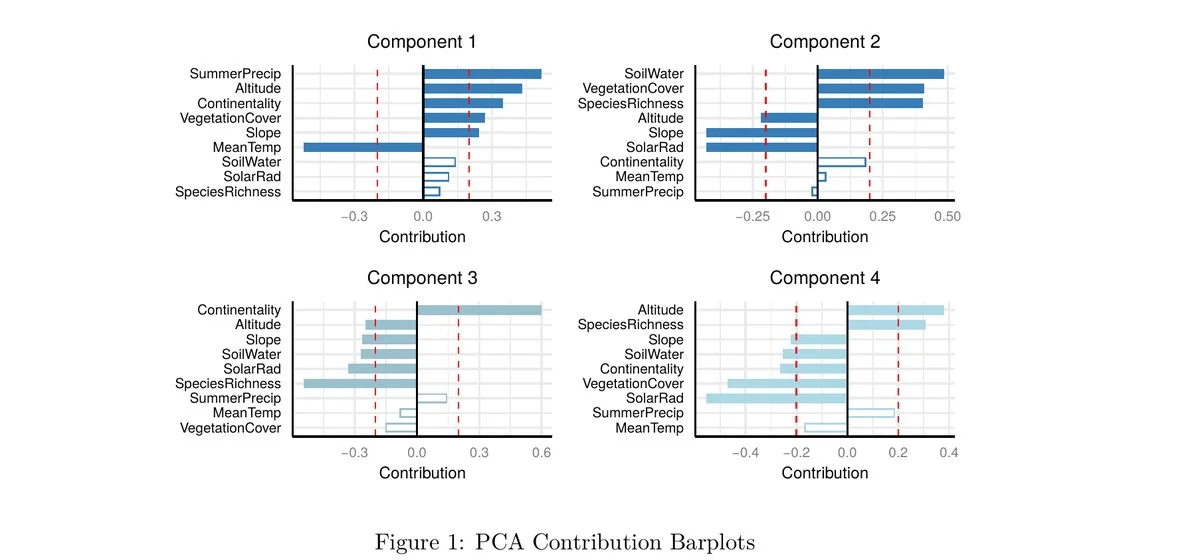
Component 1 reflects a climatic gradient of precipitation, altitude, and continentality against temperature. Component 2 reflects moisture and productivity, led by soil water, vegetation cover, and species richness. Components 3 and 4 capture more localized variation in altitude, continentality, and solar radiation.
03 / Clustering
Four environmental types, four richness patterns
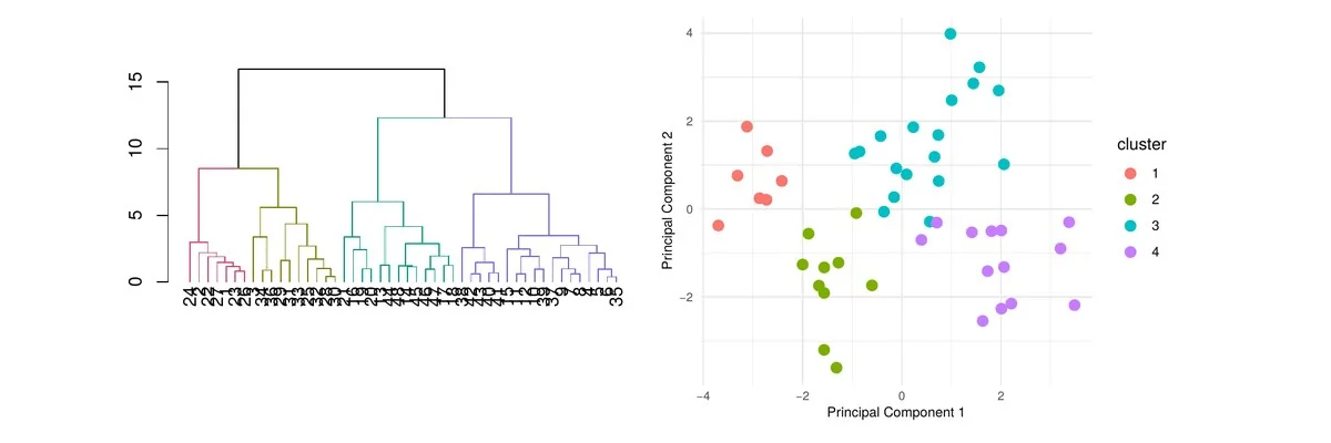
Ward's hierarchical clustering was applied to the PCA scores, with the number of clusters chosen by silhouette analysis. Four clusters gave the highest average silhouette width, at approximately 0.339.
| Cluster | Altitude | Slope | Soil water | Veg. cover | Species rich. | Mean temp |
|---|---|---|---|---|---|---|
| 1 | 42.86 | 3.10 | 23.40 | 0.10 | 17.26 | 2.33 |
| 2 | 166.00 | 15.58 | 12.91 | 0.09 | 9.88 | 1.73 |
| 3 | 190.00 | 7.23 | 44.36 | 0.50 | 16.90 | 0.81 |
| 4 | 453.85 | 16.83 | 19.02 | 0.25 | 13.21 | 0.04 |
04 / Community composition
Environment explains more than location does
A Sørensen dissimilarity matrix quantifies how different plant communities are between plot groups based on species presence. PERMANOVA then tests how much of that variation is explained by environmental variables versus site.
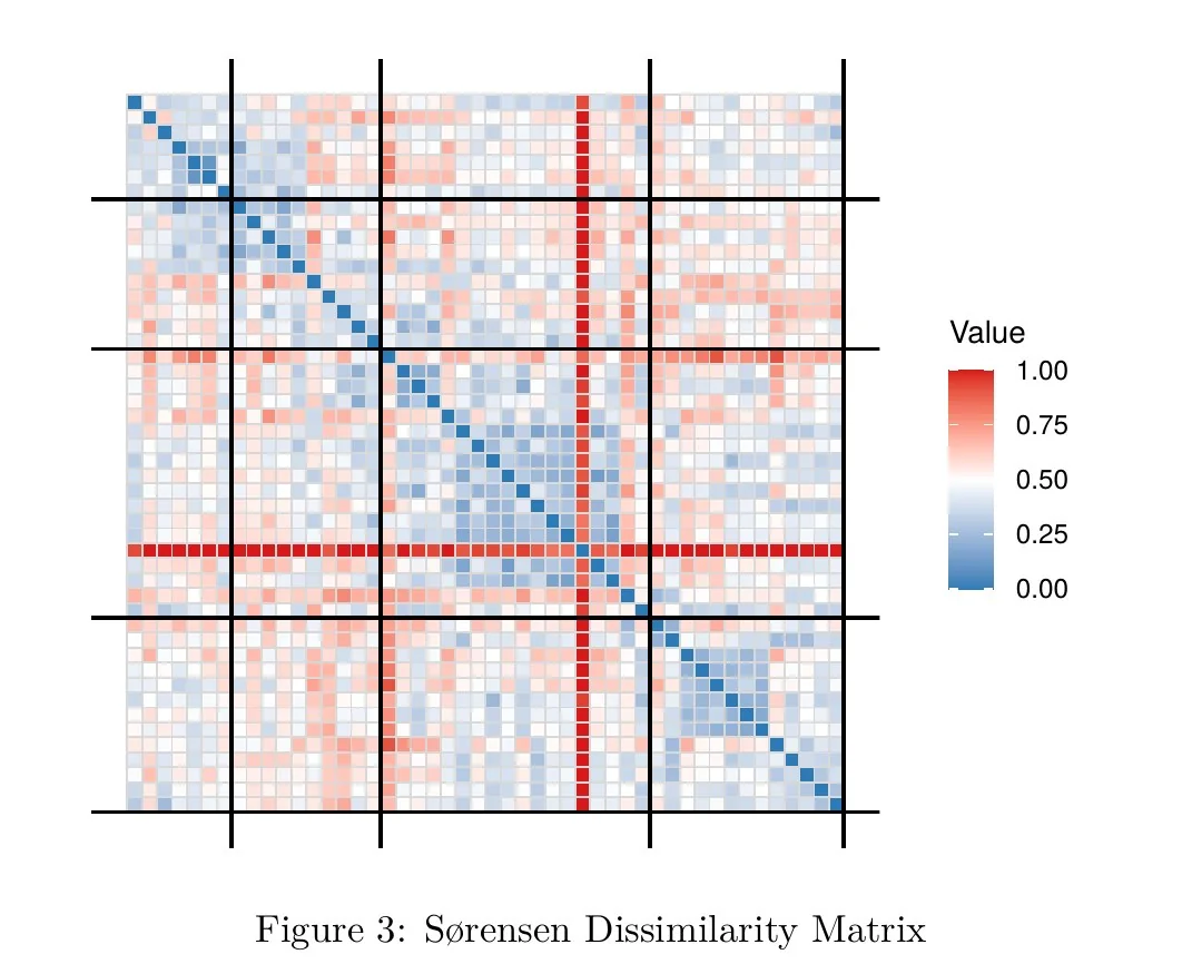
The block structure along the diagonal shows plots within the same cluster are consistently more similar to each other than to plots in other clusters, visually confirming that the environmental clusters correspond to real differences in plant community composition.
| Source | R² | p-value |
|---|---|---|
| Site | 0.254 | 0.001 *** |
| Environmental variables | 0.328 | 0.001 *** |
PERMANOVA
05 / Richness model
One predictor survives, and it is soil water
A linear mixed-effects model was fitted with environmental variables as fixed effects and site as a random effect, selected from candidate models by lowest AIC. Residual diagnostics (Q-Q plot, Shapiro-Wilk p = 0.992; residual-vs-fitted plots, Bartlett's test p = 0.738) supported the model's normality and variance assumptions.
| Term | Estimate (SE) |
|---|---|
| Intercept | 9.68 (65.58) |
| Soil water | 0.14 (0.04) *** |
| Slope | −0.04 (0.15) |
| Mean temperature | −0.12 (7.17) |
| Solar radiation | −7.85 (9.56) |
| Summer precipitation | 0.19 (2.54) |
The random effect of site (variance 2.49) is small next to the residual variance (20.68), meaning most of the unexplained variability sits within sites rather than between them. Site-level differences matter less than what is happening on the ground at each plot.
06 / By site
The same effect, but not the same strength
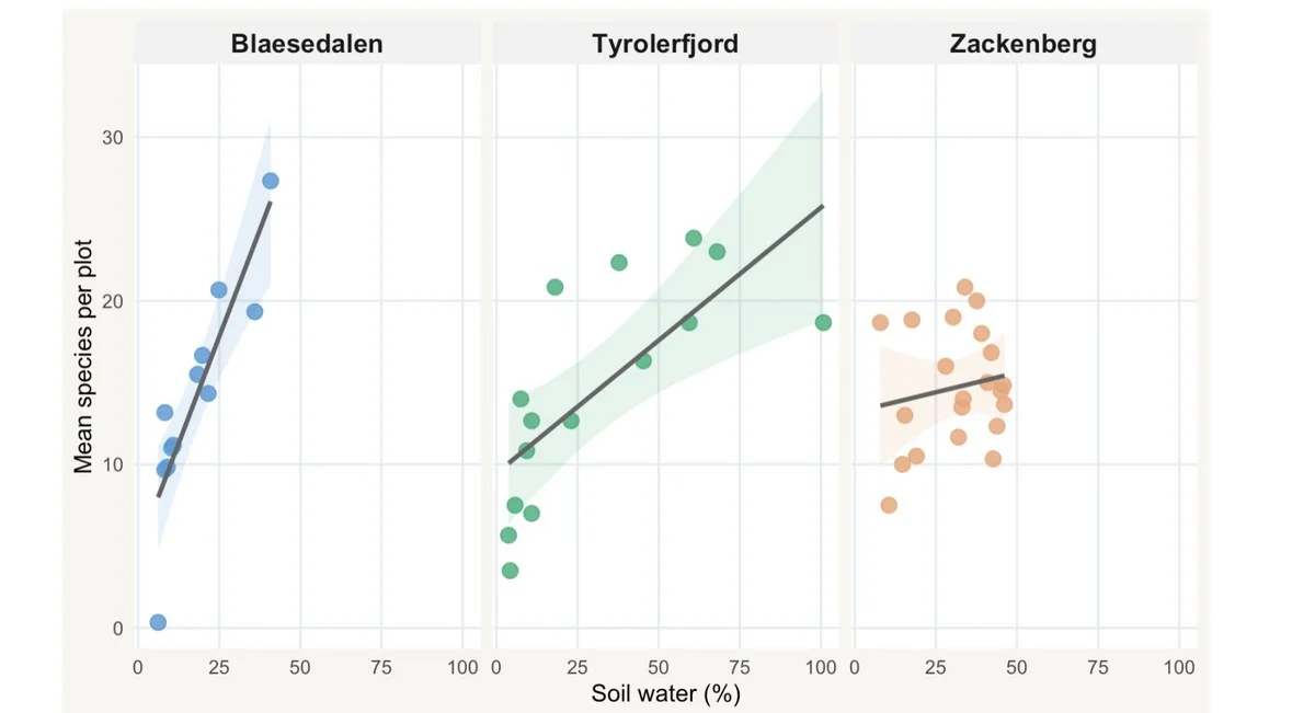
Plotting soil water against species richness separately for each site shows whether the relationship identified by the mixed model holds consistently, or depends on local context.
07 / Conclusion
Moisture, not temperature, is the limiting factor here
Environmental variation across the 48 plot groups is structured along multiple gradients rather than one dominant axis, and those gradients, not site location, are the stronger driver of plant community composition. Of everything tested in the richness model, only soil water carries a significant, consistent effect, and that effect is most pronounced in the driest environment.
What this demonstrates
- Dimensionality reduction with PCA
- Ward's hierarchical clustering with silhouette selection
- Distance-based community analysis with PERMANOVA
- Linear mixed-effects models with random effects
- AIC-based model selection
- Residual diagnostics for normality and variance
Tools and methods