Land Use, Habitat Features and Bird Diversity in Northern Italy
Count and Gamma regression across 906 survey sites, with the model family chosen by dispersion tests and diagnostics rather than by default.
Bird diversity reflects how well species thrive in their environment, and variations in land use and habitat structure can shift it substantially. This study uses a dataset of 906 observations across 38 variables, covering species richness, functional richness and functional evenness alongside environmental and habitat measures.
Pipeline
- 01
Research question
- 02
Assumptions
- 03
Model
- 04
Diagnostics
- 05
Interpretation
906
observations
38
variables
3
research questions
82.3%
deviance explained
01 / Context
Bird diversity as a measure of ecosystem health
Bird diversity reflects how well species thrive in their environment, and variations in land use and habitat structure can shift it substantially. This study uses a dataset on birds in Northern Italy, collected by a team of ecologists: 906 observations across 38 variables, covering species richness, functional richness and functional evenness alongside environmental and habitat measures.
The key predictors are dominant land use, spatial buffer zones at 100m and 250m, and habitat features including urban areas, rivers, water bodies, forests, grasslands, orchards, riparian vegetation and roads. Edge density is included to capture habitat structure.
BSR
Bird species richness
A count of species per site.
FRic
Functional richness
The spread of ecological traits.
FEve
Functional evenness
How evenly species spread across those traits.
02 / Research questions
Three questions, three models
H0 · null
The effect of being inside or outside a protected area on bird diversity is the same at the 100m and 250m scales.
H1 · alternative
The effect differs between the two scales.
H0 · null
Habitat features such as urban land cover, water presence and riparian vegetation do not significantly affect functional richness.
H1 · alternative
They do, individually or in combination.
H0 · null
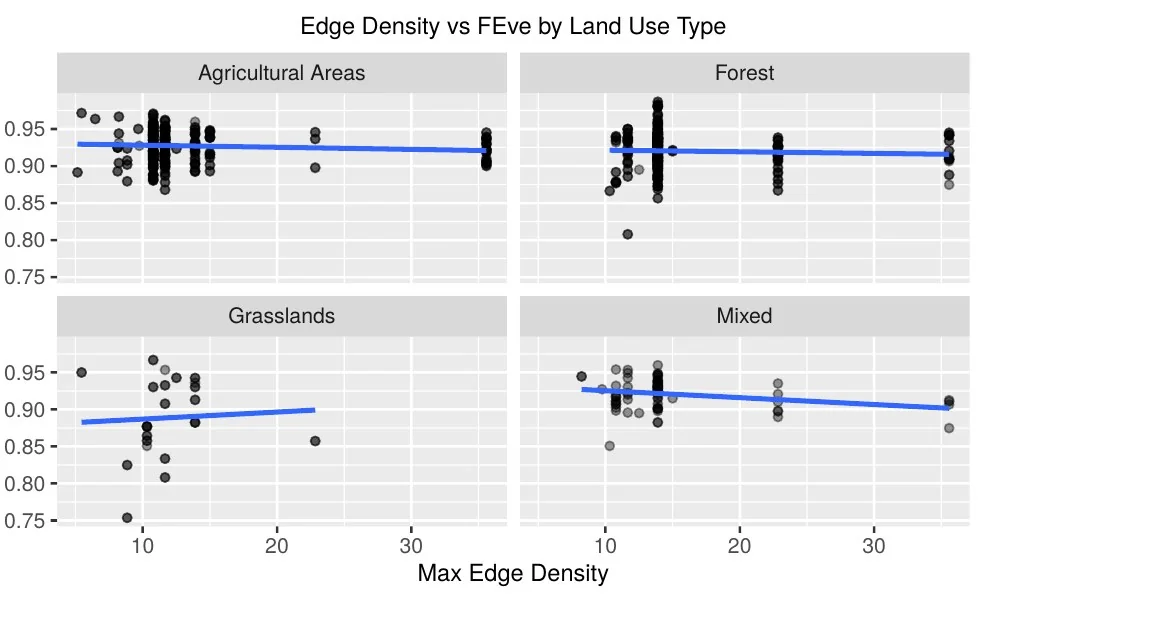
The effect of edge density on functional evenness is the same across all land use types.
H1 · alternative
It varies across land use types.
03 / Objective I
Protected areas at two spatial scales
Effects differ by scale.
Species richness is a count, so Poisson regression was the natural starting point, with log(SUM_AREA) as an offset so richness is modelled per unit area rather than as an absolute count. The dispersion test returned low p-values for both scales, meaning the equidispersion assumption failed. Both models were refitted as Negative Binomial, which lets variance exceed the mean.
Outside the buffer vs inside
−87.4%
Change in species richness rate, 100m model.
Grasslands vs agricultural
−77.5%
Forest vs agricultural
−60.2%
Outside × grasslands
+303.7%
Interaction. Outside × forest: +106.5%.
Sites outside the 100m buffer show a sharply lower richness rate, and forest and grassland sites are lower than agricultural ones. But the interactions run the other way: outside the buffer, grassland sites gain back more than fourfold. Protection matters most where the surrounding land use is poorest.
| Variable | Estimate | 95% CI | |
|---|---|---|---|
| 100m out | −2.076 | *** | −2.333, −1.819 |
| Forest | −0.921 | *** | −1.181, −0.661 |
| Grasslands | −1.491 | *** | −1.832, −1.149 |
| Mixed | −0.086 | −0.431, 0.259 | |
| out × Forest | 0.724 | *** | 0.424, 1.023 |
| out × Grasslands | 1.396 | *** | 0.799, 1.994 |
| out × Mixed | 0.232 | −0.166, 0.630 | |
| Intercept | −5.842 | *** | −6.086, −5.598 |
BSR · 100m scale · Negative Binomial · 441 observations · AIC 3214.8 · θ = 4.809 (SE 0.365). Significance: * p < 0.1, ** p < 0.05, *** p < 0.01
| Variable | Estimate | 95% CI | |
|---|---|---|---|
| 250m out | 3.883 | *** | 3.620, 4.146 |
| Forest | 0.063 | −0.206, 0.332 | |
| Grasslands | −0.538 | *** | −0.906, −0.171 |
| Mixed | 0.268 | −0.099, 0.635 | |
| out × Forest | −0.081 | −0.373, 0.212 | |
| out × Grasslands | 0.447 | * | −0.043, 0.938 |
| out × Mixed | −0.619 | *** | −1.050, −0.188 |
| Intercept | −10.395 | *** | −10.651, −10.138 |
BSR · 250m scale · Negative Binomial · 449 observations · AIC 2640.9 · θ = 11.173 (SE 1.531)
04 / Objective II
Which habitat features shape functional richness
H₀ rejected.
Functional richness is continuous and strictly positive, so a Gamma GLM with a log link was used, keeping predictions positive and treating habitat effects as multiplicative. Six models were built, from a main-effects baseline through five variants adding ecologically motivated two-way interactions such as urban with water, grassland with water, and forest with riparian vegetation.
| Variable | Estimate | 95% CI | |
|---|---|---|---|
| Water | −3.663e−04 | ** | −5.912e−04, −1.414e−04 |
| Forest | −1.883e−06 | *** | −2.573e−06, −1.193e−06 |
| Grasslands | −6.406e−06 | *** | −7.682e−06, −5.130e−06 |
| Grasslands × Water | 7.019e−09 | *** | 3.040e−09, 1.100e−08 |
| Urban × Water | 1.336e−08 | . | −4.528e−11, 2.677e−08 |
| River | −5.501e−06 | −1.575e−05, 4.747e−06 | |
| Riparian vegetation | 2.924e−06 | −1.053e−05, 1.638e−05 | |
| Orchards | 4.925e−06 | −6.541e−06, 1.639e−05 | |
| Urban | 1.517e−05 | −1.708e−05, 4.742e−05 | |
| Roads | 1.211e−05 | −3.731e−06, 2.795e−05 |
Gamma regression on functional richness, 344 observations, dispersion 0.501. Significant terms listed first. Significance: . p < 0.1, * p < 0.05, ** p < 0.01, *** p < 0.001
Water, forest and grassland area each reduce functional richness on their own, with grasslands the strongest of the three. Both interactions push the other way: where grassland meets water, and where urban land meets water, the joint presence moderates the decline. Residual deviance of 570.13 against a null deviance of 634.61 supports the fit.
05 / Objective III
Edge density and functional evenness
Failed to reject H₀.
A Gamma GLM with a log link again, this time with an interaction between maximum edge density and dominant land use, so the edge-density relationship could be read separately for each land use type. Three sparse categories, riparian vegetation or reforestation, river, and urban, were merged into a single “Other” level: the first two held one observation each and urban only 14, too few for stable interaction estimates.
| Variable | Estimate | 95% CI | |
|---|---|---|---|
| Grasslands | −0.059 | *** | −0.092, −0.026 |
| Max edge density | −0.0003 | −0.0007, 0.0001 | |
| Forest | −0.008 | −0.018, 0.002 | |
| Mixed | 0.004 | −0.014, 0.022 | |
| Other | 0.005 | −0.024, 0.034 | |
| Edge density × Forest | 0.0001 | −0.0005, 0.0007 | |
| Edge density × Grasslands | 0.001 | −0.001, 0.003 | |
| Edge density × Mixed | −0.001 | −0.003, 0.001 | |
| Edge density × Other | −0.00003 | −0.002, 0.002 | |
| Intercept | −0.072 | *** | −0.078, −0.066 |
Gamma regression on functional evenness, 906 observations, AIC −4036.97
Grasslands is the only significant term: functional evenness runs about 5.7% lower there than in the reference category. Edge density itself moves evenness by roughly 0.03% per unit, not significant at p = 0.142, and not one interaction term reaches significance. The effect of edge density does not meaningfully differ across land use types.
06 / Conclusions
What shapes a bird community
Protection works, locally
Protected areas supported greater bird diversity, and the effect was clearest at the finer 100m scale.
Habitat composition matters
Functional richness was shaped by specific features and their interactions: grasslands, forests and water bodies.
Edges, not so much
Edge density did not affect functional evenness differently across land use types.
Tools and methods
Neha Malhan · May 2026